
本 Notebook 按照 Word 实验报告要求完成,并优先参考 PDF 课本第 14 章的代码方法。
实验任务包括:
- 构建乳腺疾病识别的 AdaBoostClassifier 模型。
- 构建乳腺疾病识别的 GradientBoostingClassifier 模型。
- 构建乳腺疾病识别的 XGBClassifier 模型。
说明:Word 要求训练集和测试集比为 3:1,因此使用 test_size=0.25。PDF 课本使用的是信用卡违约或欺诈数据,与本实验数据不同,所以最终指标不会与课本数值完全一致。
import pandas as pd  # 导入 pandas 第三方包,用于读取和处理表格数据
import numpy as np  # 导入 numpy 第三方包,用于数组转换和数值计算
import matplotlib.pyplot as plt  # 导入 pyplot,用于绘制饼图、ROC 曲线和条形图
from sklearn import model_selection  # 从 sklearn 中导入 model_selection,用于拆分训练集和测试集
from sklearn import ensemble  # 从 sklearn 中导入 ensemble,用于构建 AdaBoost 和 GBDT 模型
from sklearn import metrics  # 从 sklearn 中导入 metrics,用于评估模型效果
import xgboost  # 导入 xgboost 第三方包,用于构建 XGBClassifier 模型
plt.rcParams['font.sans-serif'] = ['Microsoft YaHei']  # 设置中文字体,避免图形中的中文乱码
plt.rcParams['axes.unicode_minus'] = False  # 设置坐标轴负号正常显示
一、读取数据与预处理
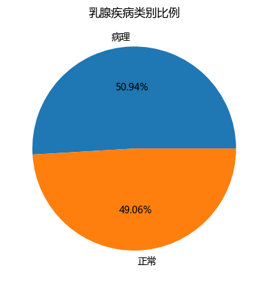
数据集第一列 type 为乳腺疾病种类,其中 Pathological 表示病理样本,Normal 表示正常样本。为了便于绘制 ROC 曲线并运行 XGBoost,将 Normal 映射为 0,将 Pathological 映射为 1。
breast = pd.read_csv(r'12-breast.csv')  # 读取 breast.csv 数据集
breast.columns = breast.columns.str.strip()  # 去除字段名两侧可能存在的空格
print(breast.head())  # 查看数据集前 5 行
print(breast.shape)  # 查看数据集的行数和列数
print(breast.type.value_counts())  # 统计不同乳腺疾病种类的样本数量
           type  impedance_zero  phase_angle  high_frequency_slope  \
0  Pathological          524.79         0.19                  0.03
1  Pathological          330.00         0.23                  0.27
2  Pathological          551.88         0.23                  0.06
3  Pathological          380.00         0.24                  0.29
4  Pathological          362.83         0.20                  0.24

   impedance_distance  area_under_spectrum  area_normalized  max_spectrum  \
0              228.80              6843.60            29.91         60.20
1              121.15              3163.24            26.11         69.72
2              264.80             11888.39            44.89         77.79
3              137.64              5402.17            39.25         88.76
4              124.91              3290.46            26.34         69.39

   distance  length
0    220.74  556.83
1     99.08  400.23
2    253.79  656.77
3    105.20  493.70
4    103.87  424.80
(106, 10)
type
Pathological    54
Normal          52
Name: count, dtype: int64
plt.axes(aspect='equal')  # 为确保饼图为圆形,设置坐标轴比例相等
counts = breast.type.value_counts()  # 统计 Pathological 和 Normal 的频数
plt.pie(x=counts, labels=pd.Series(counts.index).map({'Pathological':'病理', 'Normal':'正常'}), autopct='%.2f%%')  # 绘制样本类别比例饼图
plt.title('乳腺疾病类别比例')  # 添加图形标题
plt.show()  # 显示图形
X = breast.drop(['type'], axis=1)  # 删除因变量 type,剩余数据作为自变量 X
y = breast.type.map({'Normal':0, 'Pathological':1})  # 将类别标签数值化,其中 Normal 为 0,Pathological 为 1
X_train, X_test, y_train, y_test = model_selection.train_test_split(X, y, test_size=0.25, random_state=1234)  # 按训练集和测试集 3:1 的比例拆分数据
print(y_train.value_counts()/len(y_train))  # 输出训练集中各类别所占比例
print(y_test.value_counts()/len(y_test))  # 输出测试集中各类别所占比例
type
1    0.531646
0    0.468354
Name: count, dtype: float64
type
0    0.555556
1    0.444444
Name: count, dtype: float64
二、任务一:构建 AdaBoostClassifier 模型
AdaBoost1 = ensemble.AdaBoostClassifier()  # 构建 AdaBoostClassifier 算法的类,参数保持课本默认写法
AdaBoost1.fit(X_train, y_train)  # 使用训练数据集拟合 AdaBoostClassifier 模型
pred1 = AdaBoost1.predict(X_test)  # 使用训练好的模型对测试数据集进行预测
print('模型的准确率为:')
print(metrics.accuracy_score(y_test, pred1))  # 输出 AdaBoostClassifier 模型的准确率
print('模型的评估报告:')
print(metrics.classification_report(y_test, pred1, target_names=['Normal', 'Pathological'], zero_division=0))  # 输出 AdaBoostClassifier 模型的分类评估报告
模型的准确率为:
0.8148148148148148
模型的评估报告:
              precision    recall  f1-score   support

      Normal       0.92      0.73      0.81        15
Pathological       0.73      0.92      0.81        12

    accuracy                           0.81        27
   macro avg       0.82      0.82      0.81        27
weighted avg       0.84      0.81      0.81        27
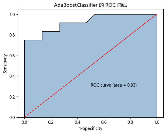
y_score1 = AdaBoost1.predict_proba(X_test)[:,1]  # 计算病理样本的概率值,用于生成 ROC 曲线的数据
fpr1, tpr1, threshold1 = metrics.roc_curve(y_test, y_score1)  # 计算 AdaBoostClassifier 模型的 FPR、TPR 和阈值
roc_auc1 = metrics.auc(fpr1, tpr1)  # 计算 AdaBoostClassifier 模型 ROC 曲线下的面积 AUC
plt.stackplot(fpr1, tpr1, color='steelblue', alpha=0.5, edgecolor='black')  # 按课本写法绘制 ROC 曲线下面积图
plt.plot(fpr1, tpr1, color='black', lw=1)  # 添加 ROC 曲线边界线
plt.plot([0,1], [0,1], color='red', linestyle='--')  # 添加随机分类器的对角线
plt.text(0.5, 0.3, 'ROC curve (area = %0.2f)' % roc_auc1)  # 在图中添加 AUC 数值文本
plt.xlabel('1-Specificity')  # 添加 x 轴标签
plt.ylabel('Sensitivity')  # 添加 y 轴标签
plt.title('AdaBoostClassifier 的 ROC 曲线')  # 添加图形标题
plt.show()  # 显示图形
importance = pd.Series(AdaBoost1.feature_importances_, index=X.columns)  # 将 AdaBoostClassifier 模型的自变量重要性转为 Series
importance.sort_values().plot(kind='barh')  # 按课本写法绘制自变量重要性的水平条形图
plt.title('AdaBoostClassifier 自变量重要性排序')  # 添加图形标题
plt.show()  # 显示图形

三、任务二:构建 GradientBoostingClassifier 模型
GBDT1 = ensemble.GradientBoostingClassifier()  # 构建 GradientBoostingClassifier 算法的类,参数保持课本默认写法
GBDT1.fit(X_train, y_train)  # 使用训练数据集拟合 GradientBoostingClassifier 模型
pred2 = GBDT1.predict(X_test)  # 使用训练好的模型对测试数据集进行预测
print('模型的准确率为:')
print(metrics.accuracy_score(y_test, pred2))  # 输出 GradientBoostingClassifier 模型的准确率
print('模型的评估报告:')
print(metrics.classification_report(y_test, pred2, target_names=['Normal', 'Pathological'], zero_division=0))  # 输出 GradientBoostingClassifier 模型的分类评估报告
模型的准确率为:
0.8148148148148148
模型的评估报告:
              precision    recall  f1-score   support

      Normal       0.92      0.73      0.81        15
Pathological       0.73      0.92      0.81        12

    accuracy                           0.81        27
   macro avg       0.82      0.82      0.81        27
weighted avg       0.84      0.81      0.81        27
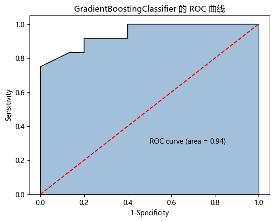
y_score2 = GBDT1.predict_proba(X_test)[:,1]  # 计算病理样本的概率值,用于生成 ROC 曲线的数据
fpr2, tpr2, threshold2 = metrics.roc_curve(y_test, y_score2)  # 计算 GradientBoostingClassifier 模型的 FPR、TPR 和阈值
roc_auc2 = metrics.auc(fpr2, tpr2)  # 计算 GradientBoostingClassifier 模型 ROC 曲线下的面积 AUC
plt.stackplot(fpr2, tpr2, color='steelblue', alpha=0.5, edgecolor='black')  # 按课本写法绘制 ROC 曲线下面积图
plt.plot(fpr2, tpr2, color='black', lw=1)  # 添加 ROC 曲线边界线
plt.plot([0,1], [0,1], color='red', linestyle='--')  # 添加随机分类器的对角线
plt.text(0.5, 0.3, 'ROC curve (area = %0.2f)' % roc_auc2)  # 在图中添加 AUC 数值文本
plt.xlabel('1-Specificity')  # 添加 x 轴标签
plt.ylabel('Sensitivity')  # 添加 y 轴标签
plt.title('GradientBoostingClassifier 的 ROC 曲线')  # 添加图形标题
plt.show()  # 显示图形
四、任务三:构建 XGBClassifier 模型
XGBoost1 = xgboost.XGBClassifier(eval_metric='logloss')  # 构建 XGBClassifier 算法的类,保留默认参数并设置评估指标以适配当前版本
XGBoost1.fit(X_train, y_train)  # 使用训练数据集拟合 XGBClassifier 模型
pred3 = XGBoost1.predict(X_test)  # 使用训练好的模型对测试数据集进行预测
print('模型的准确率为:')
print(metrics.accuracy_score(y_test, pred3))  # 输出 XGBClassifier 模型的准确率
print('模型的评估报告:')
print(metrics.classification_report(y_test, pred3, target_names=['Normal', 'Pathological'], zero_division=0))  # 输出 XGBClassifier 模型的分类评估报告
模型的准确率为:
0.7777777777777778
模型的评估报告:
              precision    recall  f1-score   support

      Normal       0.85      0.73      0.79        15
Pathological       0.71      0.83      0.77        12

    accuracy                           0.78        27
   macro avg       0.78      0.78      0.78        27
weighted avg       0.79      0.78      0.78        27
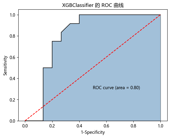
y_score3 = XGBoost1.predict_proba(np.array(X_test))[:,1]  # 计算病理样本的概率值,用于生成 ROC 曲线的数据
fpr3, tpr3, threshold3 = metrics.roc_curve(y_test, y_score3)  # 计算 XGBClassifier 模型的 FPR、TPR 和阈值
roc_auc3 = metrics.auc(fpr3, tpr3)  # 计算 XGBClassifier 模型 ROC 曲线下的面积 AUC
plt.stackplot(fpr3, tpr3, color='steelblue', alpha=0.5, edgecolor='black')  # 按课本写法绘制 ROC 曲线下面积图
plt.plot(fpr3, tpr3, color='black', lw=1)  # 添加 ROC 曲线边界线
plt.plot([0,1], [0,1], color='red', linestyle='--')  # 添加随机分类器的对角线
plt.text(0.5, 0.3, 'ROC curve (area = %0.2f)' % roc_auc3)  # 在图中添加 AUC 数值文本
plt.xlabel('1-Specificity')  # 添加 x 轴标签
plt.ylabel('Sensitivity')  # 添加 y 轴标签
plt.title('XGBClassifier 的 ROC 曲线')  # 添加图形标题
plt.show()  # 显示图形
result = pd.DataFrame({'模型':['AdaBoostClassifier', 'GradientBoostingClassifier', 'XGBClassifier'], '准确率':[metrics.accuracy_score(y_test, pred1), metrics.accuracy_score(y_test, pred2), metrics.accuracy_score(y_test, pred3)], 'AUC':[roc_auc1, roc_auc2, roc_auc3]})  # 汇总三个模型的准确率和 AUC
result  # 显示模型对比结果
| 模型 | 准确率 | AUC | |
|---|---|---|---|
| 0 | AdaBoostClassifier | 0.814815 | 0.925000 |
| 1 | GradientBoostingClassifier | 0.814815 | 0.944444 |
| 2 | XGBClassifier | 0.777778 | 0.802778 |
五、实验结果分析
从本次实验结果看,乳腺数据集中 Pathological 和 Normal 的样本比例约为 50.94% 和 49.06%,不存在 PDF 课本信用卡案例中严重类别不平衡的问题,因此未使用 SMOTE 处理。
本实验的结果与 PDF 课本示例结果不同,主要原因是:PDF 使用的是信用卡违约或信用卡欺诈数据集,而 Word 要求使用 breast.csv 乳腺疾病数据集;数据规模、字段含义、类别比例和训练测试拆分比例均不同,因此准确率、分类报告和 AUC 不可能与课本示例数值完全一致。
在当前训练测试拆分下,三个集成模型都能够完成乳腺疾病识别任务。医学识别场景中,病理样本的漏判风险更高,因此除了总体准确率,也应重点关注 Pathological 类别的 recall。
六、思考题
AdaBoostClassifier、GradientBoostingClassifier、XGBClassifier 都属于集成学习中的提升类算法,基本思想都是将多个弱学习器组合成一个更强的分类模型。
AdaBoostClassifier 通过提高上一轮被错分样本的权重,使后续弱分类器更加关注难分类样本。GradientBoostingClassifier 则从损失函数的负梯度方向逐步拟合残差,本质上是不断修正前一轮模型的误差。XGBClassifier 是对 GBDT 的工程化和算法层面改进,引入了正则化、二阶梯度信息、列采样、缺失值处理和更高效的计算机制。
三者的联系是都采用逐轮迭代、多个基学习器叠加的提升思想;区别在于 AdaBoost 主要调整样本权重,GBDT 主要拟合损失函数梯度,XGBoost 在 GBDT 基础上进一步优化目标函数、正则化和计算效率。